Data combinations
The following data combinations are available: average, sum, RMS deviation, and only for 1D: classical PCA, cumulative PCA, target transformation and MCR-ALS. If the abscissas of the involved 1D datasets differ, interpolation can be optionally applied. These operations are performed on all arrays defined in the node.arrays dictionary and result in the creation of one or more new datasets.
Average, sum, rms deviation
These combinations generate a single new data item from multiple user-selected datasets.
PCA: classic and cumulative
The user specifies a 1D array name for PCA analysis. These arrays from \(n\) selected data items may have different lengths. In such cases, they are interpolated onto the abscissa grid of the first selected dataset. The \(n\) arrays form an \(m×n\) data matrix \(D = \begin{bmatrix} \mathbf{d}_1 & \mathbf{d}_2 & \dots & \mathbf{d}_n \end{bmatrix}\).
For the covariance matrix \(D^TD\), the eigenvalues \(\lambda_j\) and corresponding eigenvectors \(\mathbf{e}_j\) are computed and sorted in descending order of \(\lambda_j\) with \(\lambda_1\) being the largest. The following identity always holds: \(\sum_{j=1}^n \mathbf{e}_j \mathbf{e}_j^T = \mathbf{1}\).
If only \(N<n\) data vectors are linearly independent, the sum can be truncated at \(j=N\), while still satisfying \(\sum_{j=1}^N \mathbf{e}_j \mathbf{e}_j^T = \mathbf{1}\). In this case \(\lambda_j=0\) for all \(j > N\). In practice, truncation is applied such that \(D\sum_{j=1}^{N}\mathbf{e}_j\mathbf{e}^T_j\) reproduces \(D\) within the noise level. Equivalently, the discarded contribution \(D\sum_{j=N+1}^{n}\mathbf{e}_j \mathbf{e}^T_j\) remains within the noise.
ParSeq does not currently provide dedicated tools for estimating noise levels. Consequently, direct comparison of the truncated contribution with the noise is not implemented as a general feature. Instead, (a) the scree plot and (b) Malinowski’s IND function [IND] are provided to assist in determining the appropriate value of \(N\).
The data matrix admits two PCA representations:
Here, \((k)\) denotes the \(k\)th principal component. In both representations, the first PCA component is the average of all spectra. Subsequent components represent deviations from this average: in the classical PCA, each component describes an individual deviation mode, whereas in the cumulative PCA, the components represent progressively accumulated deviations added to the average.
E R Malinowski, Anal. Chem. 49 (1977) 606.
Target transformation
From \(n\) selected basis (reference) 1D datasets, an \(m×n\) basis matrix is constructed: \(B = \begin{bmatrix} \mathbf{d}_1 & \mathbf{d}_2 & \dots & \mathbf{d}_n \end{bmatrix}\). If the array length \(m\) differs among the \(n\) basis spectra, they are interpolated to match the grid of the first dataset.
If the basis spectra are linearly independent then the covariance matrix \(B^TB\) (of size \(n×n\)) has full rank \(n\) and its inverse \((B^TB)^{-1}\) exists. The matrix \(B(B^TB)^{-1}B^T\) is an orthogonal projector onto the subspace spanned by the basis spectra, since it is idempotent (equal to its square). Consequently, a spectrum \(\mathbf{d}\) belongs to this subspace if and only if \(B(B^TB)^{-1}B^T\mathbf{d}=\mathbf{d}\).
In practice, one verifies whether \(B(B^TB)^{-1}B^T\mathbf{d}\) reproduces \(\mathbf{d}\) within the noise level. In ParSeq, the inverse covariance matrix is computed via the eigenvalues \(\lambda_j\) and eigenvectors \(\mathbf{e}_j\) of \(B^TB\): \((B^TB)^{-1} = \sum_j\lambda_j^{-1}\mathbf{e}_j\mathbf{e}^T_j\). This approach also enables inspection of the eigenvalues to assess the linear independence of the basis spectra.
MCR-ALS
The Multivariate Curve Resolution–Alternating Least Squares (MCR-ALS) method [Tauler-ALS] enables the decomposition (with potentially many valid solutions) of an \(m×n\) data matrix \(D\) into the product of \(N\) basic components collected in the matrix \(S\) (\(m×N\)) and \(N\) concentration profiles collected in the matrix \(C\) (\(n×N\)):
This section describes the ParSeq implementation of MCR-ALS.
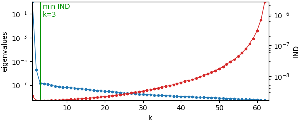 Eigenvalue analysis of 70 XANES spectra during gas switching.
Eigenvalue analysis of 70 XANES spectra during gas switching.
The first step is to determine the number of basic components, \(N\). This can be guided by examining the scree plot (a plot of eigenvalues vs their ordinal index) and Malinowski’s IND function. In practice, however, these methods often do not yield a definitive result, and the value of \(N\) is typically guessed.
The second step is to obtain an initial estimate of \(S\). Often, one component (i.e., one column of \(S\)) is known from the sample history and can be taken as either the initial or the final spectrum in a measurement series. The remaining columns can be determined by identifying spectra that exhibit the largest deviation from the components already defined. This is achieved by subtracting the target transformation of \(D\) from \(D\) and selecting the column with the largest norm. That column of \(D\) is then used as the next initial column of \(S\).
The next stage consists of two alternating matrix transformations that are applied iteratively to compute: (a) \(C\) from \(D\) and \(S\), according to the transposed Eq. (1) and (b) \(S\) from \(D\) and \(C\), according to Eq. (1). The transformations are given by \(C = D^TS(S^TS)^{-1}\) and \(S = DC(C^TC)^{-1}\). After each transformation, common constraints are enforced: non-negativity of \(C\) and optionally \(S\), and mass balance (i.e. the sum of each row of \(C\) equals 1). Prior to applying any constraints, the columns of \(C\) and \(S\) are simultaneously sorted by the integrated column weights of \(C\). Additionally, prior to applying the mass balance constraint, lower and/or upper bounds may be imposed on individual columns of \(C\). These alternating transformations are repeated until convergence is achieved. If \(S^TS\) or \(C^TC\) becomes singular, the iterative scheme fails to converge to a solution.
The final step is to estimate the uncertainties in \(S\) and \(C\). One possible approach is to perform linear combination fitting (LCF) using the obtained \(S\) as the basis set. However, the fit quality is typically dominated by systematic uncertainties, which leads to a significant underestimation of the error bars. For this reason, the LCF approach was discarded in ParSeq.
Instead, ParSeq employs the rotation-matrix approach of [Tauler-boundaries], although with a different implementation. Equation (1) can be rewritten by inserting an \(N\times N\) identity matrix \(I\) and decomposing it into the product of a matrix \(T\) (initially arbitrary, only invertible) and its inverse \(T^{-1}\). These two matrices define new effective matrices \(S'\) and \(C'\):
We require the matrices \(S'\) and \(C'\) to retain the same physical meaning as \(S\) and \(C\). To preserve the normalization of the columns of \(S'\), each column of \(T\) must sum to unity (column-normalized). Likewise, to preserve mass balance in \(C'\), each row of \(T^{-1T}\) (column of \(T^{-1}\)) must also be normalized. In fact, satisfying either condition automatically guarantees the other, as follows from the theorem that the inverse of a square column-normalized matrix is itself column-normalized.
The inverse of a dense positive matrix generally contains negative elements. Consequently, it is impossible to enforce non-negativity simultaneously in both \(S'\) and \(C'\), which can be addressed by interpreting negative values in \(C'\) (concentrations) or \(S'\) (spectra) as carrying the same meaning as their positive counterparts.
Random realizations of \(T\) generate an ensemble of matrices \(S'\) and \(C'\), enabling the estimation of uncertainties in \(S\) and \(C\). In ParSeq, \(T\) is sampled as a non-negative column-normalized matrix, thereby preserving both the sign and the normalization of the spectra in \(S' = ST\). The corresponding concentration matrix is obtained as \(C' = {\rm abs}(CT^{-1T})\), followed by row normalization to restore mass balance. Positive and negative RMS deviations from \(S\) and \(C\) are then computed from an ensemble of random realizations of \(T\) (1000 by default).
R Tauler, A Smilde, BR Kowalski, J. Chemometrics 9 (1995) 31.
R Tauler, J. Chemometrics 15 (2001) 627.
Examples of MCR-ALS
 70 XANES spectra during gas switching.
70 XANES spectra during gas switching.
1. Ni-containing catalyst: Oxidation.
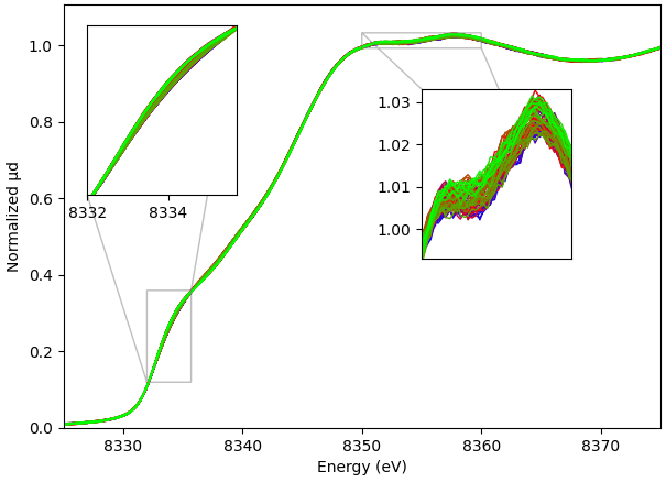
A series of operando spectra of a Ni-containing catalyst measured in a capillary cell at the Balder/MAX-IV beamline during gas switching [Ni-MCR-ALS]. The dataset consists of 63 XANES spectra showing subtle variations in both the edge position and the white-line region, see on the right.
The scree plot and Malinowski’s IND function suggest that the number of independent components is 3. This would imply transitions between two main states with a third, likely transient, intermediate state. However, the ALS analysis does not yield a physically meaningful concentration profile \(C_3\) and a well-defined component \(S_3\). Notably, there is a large difference spanning several orders of magnitude between the first and second eigenvalues, see the scree plot above, while the gap between the second and third is much smaller. This indicates that the second and third components are not well separated. Consequently, the number of independent components was set to 2.
 MCR-ALS of 70 XANES spectra during gas switching. S matrix.
MCR-ALS of 70 XANES spectra during gas switching. S matrix.
 MCR-ALS of 70 XANES spectra during gas switching. C matrix.
MCR-ALS of 70 XANES spectra during gas switching. C matrix.
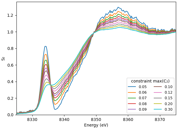
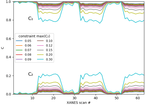
The solutions for \(S\) and \(C\) are not unique, as illustrated by the accompanying figures. In this example, a low-pass constraint is applied to \(C_2\) . Varying this constraint leads to different solutions for both \(C\) and \(S\). One might expect that these alternative solutions could be distinguished by the norm of the residual \(D - SC^T\). However, this norm is typically orders of magnitude smaller than the noise level, making all such solutions effectively equivalent in terms of fit quality. Therefore, selecting the most appropriate solution requires additional chemical or physical insight beyond the mathematical decomposition.
If the ALS solution is not unique, does it still have value? In the two-dimensional space defined by basic spectra and their concentrations, all admissible points are a priori valid solutions. The MCR-ALS method reduces this space to a one-dimensional manifold (a line). If this line intersects known reference spectra, the interpretation becomes straightforward, and the method is clearly valuable. Even when the resulting components \(S\) do not resemble any known reference spectra, further discrimination may still be possible using computational spectroscopy or other complementary techniques. Thus, even a continuum of possible solutions can provide meaningful insight and may still be scientifically valuable and publishable.
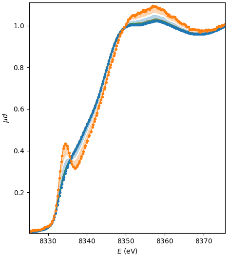 MCR-ALS analysis of 63 Ni-K spectra, S matrix. The main pure
component 1 (blue) is metallic, and the pure component 2 (orange) is
oxidic, shifted to higher energy.
MCR-ALS analysis of 63 Ni-K spectra, S matrix. The main pure
component 1 (blue) is metallic, and the pure component 2 (orange) is
oxidic, shifted to higher energy.MCR-ALS analysis of 63 Ni-K spectra, S matrix. The main pure component 1 (blue) is metallic, and the pure component 2 (orange) is oxidic, shifted to higher energy.
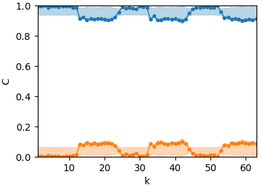 MCR-ALS analysis of 63 Ni-K spectra, C matrix. The main pure
component 1 (blue) is metallic, and the pure component 2 (orange) is
oxidic, shifted to higher energy.
MCR-ALS analysis of 63 Ni-K spectra, C matrix. The main pure
component 1 (blue) is metallic, and the pure component 2 (orange) is
oxidic, shifted to higher energy.MCR-ALS analysis of 63 Ni-K spectra, C matrix. The main pure component 1 (blue) is metallic, and the pure component 2 (orange) is oxidic, shifted to higher energy.
For a low-pass constraint \(C_2<0.1\), the resulting matrices \(S\) and \(C\) are displayed on the left and right, with the RMS deviation bands plotted by shaded colors.
The shown example can be scrutinized by running the script
parseq/tests/test_MCRWidget.py and/or by loading the ParSeq-XAS project
file parseq_XAS/saved/mcr.pspj.
N Kosinov (2026) private communication, unpublished.
2. Ce-containing catalyst: Reduction
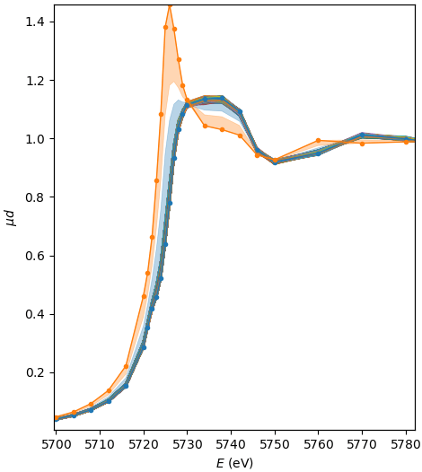 MCR-ALS analysis of 1102 Ce-L3 spectra, S matrix. The main pure
component 1 (blue) is Ce4+, and the pure component 2 (orange) is Ce3+,
shifted to lower energy.
MCR-ALS analysis of 1102 Ce-L3 spectra, S matrix. The main pure
component 1 (blue) is Ce4+, and the pure component 2 (orange) is Ce3+,
shifted to lower energy.MCR-ALS analysis of 1102 Ce-L3 spectra, S matrix. The main pure component 1 (blue) is Ce4+, and the pure component 2 (orange) is Ce3+, shifted to lower energy.
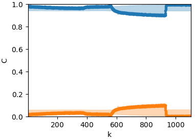 MCR-ALS analysis of 1102 Ce-L3 spectra, C matrix. The main pure
component 1 (blue) is Ce4+, and the pure component 2 (orange) is Ce3+,
shifted to lower energy.
MCR-ALS analysis of 1102 Ce-L3 spectra, C matrix. The main pure
component 1 (blue) is Ce4+, and the pure component 2 (orange) is Ce3+,
shifted to lower energy.MCR-ALS analysis of 1102 Ce-L3 spectra, C matrix. The main pure component 1 (blue) is Ce4+, and the pure component 2 (orange) is Ce3+, shifted to lower energy.
A series of 1102 Ce L3-edge XANES spectra of a 1.5 wt% Pt/CeO2 catalyst during cyclic reduction and oxidation conditions [Ce-MCR-ALS].
The shown example can be scrutinized by running the script
parseq/tests/test_MCRWidget.py and/or by loading the ParSeq-XAS project
file parseq_XAS/saved/mcr-ceria-big.pspj. Warning: This is a big dataset!
Data loading can take a minute.
A Martini (2026), private communication. A similar MCR analysis is present in Fig. 21 in [Martini_Crystals]. Dataset from [Guda_JSR].
A Martini and E Borfecchia, Crystals 10 (2020) 664.
A Guda et al, J. Synchrotron Rad. 25 (2018) 989.
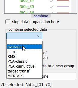
Data combination widget
 Data combination widget
Data combination widget
The widget “combine” can be found in the “Data” splitter under the list of all data items.
Average, sum, rms deviation
Select one or more data items, select a combination type and press “Combine” button. A new data item will be created and placed after the selected parental data.
PCA
For a selected set of data, a plot window appears at the bottom of the widget, displaying both a scree plot and the IND function. Use these plots to choose the desired number of components, then click the “Combine” button. For each parent data item, a new group will be created containing the PCA components of the specified 1D array.
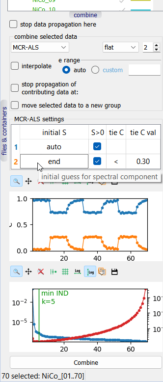 Data combination widget with MCR-ALS settings
Data combination widget with MCR-ALS settings
Target transformation
Select a data item and choose the combination type “target-transformation”. Then click the “Combine” button. A data selection dialog will appear, allowing to choose a set of basis spectra. After clicking “Apply”, a new data item will be created under the original one, containing the resulting target transformation. Compare this new item with the original data.
MCR-ALS
For a selected set of examined data and a given value of \(N\), the widget provides a table of MCR-ALS settings, including definitions of the initial \(S\) and optional constraints on \(S\) and \(C\).
Note that the choice of the abscissa range is an additional parameter that can influence the MCR-ALS solution. The combination widget includes a range selector to help define an appropriate spectral interval.
The resulting \(C\) is displayed at the bottom of the widget, while the corresponding \(S\) is shown in the main node plot. After clicking the “Combine” button, a new data group is created containing the columns of \(S\) as new spectra.